Chapter 10 Neural Networks
Contents:
10.1 Introduction
10.1.1 Biological neurons and their models
Biological brains are excellent at recognizing patterns in a noisy image. They often learn from examples of such patterns, just as we learned to recognize letters and numbers when we were young,
we didn't need any symbolic descriptions of how the letter or number must look like. On the other hand, pattern recognition using computer programs is very slow and tiring. Typed text, with a well
defined and constant shape of characters can be recognized pretty well, but recognition of handwriting is hardly used.
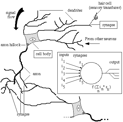 |
It may be helpful to have a look at human brains to look for information which we can use in some form or another in computer programs. In the nervous system, electrical pulses that run over the
axon of a nervous cell transmiting signals between nervous cells, called neurons. The pulses are made by ions in motion, with a speed of up to 100 m/s; contrary to electrical current where the
electrons are in motion. Axons typically branch out, and each branch comes very close to another type of offshoot from a cell, called a dendrite. The contact point is called a synaptic gap or just
synapse. An axon pulse releases chemical substances, the neurotransmitters, which clamp onto the dendrite receptors and help ions in or out of the dendrite.
|
Because of that, the electrical current in the neurons fluctuates, whereby the effects of several receptors and dendrites can primarily be summed up linearly. When the charge in a cell increases
beyond a certain threshold value, the axon hillock will send a pulse over the axon. This happens when Na+ and K+ ions enter and leave the cell. When the concentrations of
Na+, K+ and Cl- ions in the cell have been restored by a metabolic process, the Na/K pump, the entire process can repeat itself. Each neuron works independently of
all other neurons; with exception of the cell's metabolic processes, the making and breaking down of the neurotransmitters, supply of building materials and the discharge of waste materials through
the blood veins. The human central nervous system is composed of the bone marrow, the brainstem, the small brains and the large brains, which is itself composed of the thalamus, the hypothalamus and
the cortex, and can be distinguished into 6 layers.
A simple model of a neuron is given above. The input values in enter via synapses. The influence of the synapse is given by a value sn where in is multiplied. The
total value of the neuron then becomes:  n sn• in. The
output of the neuron is the function f released on that value and is then passed on to the other neurons. A neural network model is made up of several neurons connected together and an indication on
how the model shall learn, for example by changes in the sns, the external input.
Neural Networks (NN) are thus models with properties such as calculation, recognition, association, learning, etc.:
- with many units, the neurons, that work in a parallel manner and possibly synchronized, where simple mathematical calculations take place.
- with a large amount of connections between the neurons.
- with learning rules. The parameters, that determine the behavior by especially the strength of the connections, is determined by the offered examples.
- with biological brains as a good example ( 1011 neurons, 1015 connections or synapses, 100 - 500 Hz ).
- used to:
- describe and study the functioning of biological neurons and brains.
- solve practical problems effectively, independent of the functioning of the biological systems.
- they are essentially parallel and yield good possibilities for the use of parallel computer systems.
A definition from Kohonen ( Neural Networks, Vol 1 1988):
"Artificial Neural Networks are massively parallel interconnected networks of simple ( usually adaptive) elements and their hierarchical organizations which are intended to interact with
the objects of the real world in the same way as biological nervous systems do."
For neural networks many terms and their abbreviations are used, depending on which aspect one chooses: Neurocomputing, Connectionist models, Parallel Distributed Programs (PDP), (Artificial)
Neural Networks (ANN or NN) and Neuro Informatics, to name just a few.
10.1.2 Computer Science research
The NN models are studied using mathematical and computer science methods, but also by evaluation or simulation of it on serial and parallel computers. This requires immense calculation capacity
just to use a relatively small mode, up to one thousand neurons.
 |
Within informatics we are searching for methods to accelerate the simulation of NNs on parallel computer systems. Also important are the resources for the (graphical) construction and description
of NNs and for the visualization of the simulation and the results thereof. A lot of computer science research concentrates on the use of NNs for pattern recognition, such as for speech, handwriting
and image recognition; and to control apparatuses such as robots. Also being researched is appropriate architecture for the execution of NNs, such as parallel machines and the direct implementation
of NN models in VLSI hardware.
|
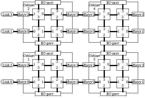 |
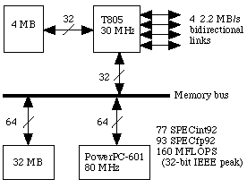
Within ITA we used a PowerXplorer parallel computer systems for research and parallel implementation of neural networks and for research into the use of NNs for satellite photos. This PowerXplorer
is built up out of nodes, each composed of a calculation and a communication microprocessor and memory, of which 16 are connected to each other.
Primarily, we now use serial SUN workstations for the use of neural networks for pattern recognition. Both serial and parallel implementation use the same format for I/O data files and the storing
of network parameters. Both implementations can be used for the same practical applications.
|
 |
The PowerXplorer is connected to a SUN machine. The program development, compilation and linking is completely executed on the SUN. A maximum of four users can claim some nodes to execute a
program.
|
10.1.3 Historical Overview
1943
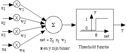 |
McCulloch and Pitts laid down the basis for the design of neural networks. They showed that the neuron-type elements are capable of general calculations. They introduced the Logic Threshold Unit
(LTU) with binary input and output and a threshold function with threshold  which works on the
activation (as just mentioned) of the neuron. which works on the
activation (as just mentioned) of the neuron.
|
1949
Hebb introduced "learning" with the suggestion that synapses are the location of biological learning. Synapses that are often active have a larger chance of becoming active again. This idea led to
the learning rule of Hebb:
wj(t+1) = wj(t) +  xj y with
  a parameter
1958
Rosenblatt developed the perceptron, in was composed of one layer with LTUs and could deal with simple pattern recognition problems. Widrow introduced the Adaptive Linear Combiner and the Adaline
(Adaptive linear neuron), frequently used in signal processing. He also introduced the supervised learning rule:
wj(t+1) = wj(t) +  xj (t-y ) with t the desired value of
y at x
composed of xp and tp, and applied to each offering of a pattern p.
1969
 |
Minsky and Papert showed that a one-layer perceptron network cannot solve certain problems. They thought that a network with more layers, to solve such problems, would not be capable of learning
properly; years later this was found to be incorrect.
|
The decision point, there where the output goes from 0 to 1, of a LTU is given by  k
xkwk =
  , which defines a hyper-plane that is spanned in the n-dimensional space by
x. With 2 inputs this becomes a line, as shown in the figure above. The desired output of AND and OR functions can be separated by a line, however those of the XOR cannot. For that we need two
LTUs and one LTU that works on the output of the first two.
1975
Fukushima designed the cognitron and later the neo-cognitron, a generalization of the multi layer perceptron with "unsupervised" learning capabilities.
1982
Hopfield, a physicist, used methods from theoretical physics, especially statistical physics, to design an algorithm for selective storage and looking up of patterns in a 1-layer network.
1984
Kohonen designed the "topology preserving maps" or "self-organizing feature maps" with Learning Vector Quantization learning rules. This has successfully been applied to the translation of continuous
speech to phonemes in Finish and Japanese.
1986
Rummelhart and McClelland, in their 3-part Parallel Distributed Programming, designed multi-layer feed-forward networks with back-propagation learning rules, an extension of the delta-learning rule.
This got a lot of attention from psychologists. These NNs can solve any problem that can be defined formally. However, there are problems:
- learning is slow and with a poor convergence.
- the learning rules are not biologically plausible.
- there is no measurement for deciding when the system has learned a task.
Despite this, it is still the most used NN model.
1987
Carpenter and Grossberg were the primary designers of the "adaptive resonance" theory (ART), an "unsupervised" learning model that is biologically plausible.
10.2 Models
10.2.1 Components of Neural Networks
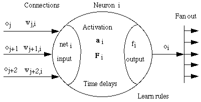 |
Neural networks are often decomposed into the following components:
- Processing units
These neurons receive inputs from other units, calculate an output and send that to other neurons. Often there are input and output neurons, that connect it to the world outside, and internal or
"hidden" neurons. The values of the signals are often restrained to the interval [0,1] or [-1,1].
|
- Activation state
These are internal states of neurons that change with time: ai(t+1) = F ( ai(t), neti(t) )
where neti is a vector that is calculated from the input values o. This is often only a scalar weighted sum of inputs, or the Euclidic distance between the input and
the weighted vector:
neti(t) =  j ( wj,i (t) * oj(t) ) or
neti(t) = || w(t) - o(t) || 2 =
  j ( wj,i (t) -
oj(t) ) 2
Often ai is also a scalar ai, that is equal to neti. But one can also model multiplicative dendrite effects with it, or time integration:
neti(t) =  j
j  (wj,i(t) * oj(t-
 ) ) d
) ) d  . Also one can build in memory to model refractory periods with it.
- Output
This is an activation function: oi (t) = f( ai(t) ) or delayed oi (t) = f( ai(t - t) )
t) )
With a Euclidic distance for neti, often a Gaussian function of neti is used. The output function can also be stochastic, the output is then 1 with a probability according to
the curves above.
- Connections
Connections between neurons can be specified, often in a weighted matrix w, wi,j indicates the strength of the connections between the neurons i and j. A positive weight
describes an exiting, a negative weight an inhibiting connect. A large amount of structures is possible, where often only a part of w is occupied.
- Learning rules
These describe the change in time of the parameters, usually affecting only the weighted matrix w and the parameters of the output function such as  and
and  . But also internal neuron functions (F and
f) and network structures (adding neurons) can change. Often learning is an activity on its own, first a task is learned which can later be executed repetitively.
10.2.2 Structures
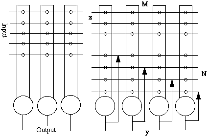
A basic structure is the "crossbar" switch.
Following in complexity is the use of lateral feedback. For the feedback unit the following holds:
dy/dt = f (x, y, M, N) , the relaxation equation
dM/dt = g (x, y, M) , the adaptation equation
dN/dt = h (y, N) , the adaptation for feedback.
In general one can see (parts of) networks as "feed-forward" ( the output signals influence the input signals neither directly nor indirectly ) or "feedback". The feedback can occur on a local or
global level.
We also concentrate on networks (for example Hopfield) which have no explicit input or output signals. Often one looks at the change in state of the neurons, from an initial to a final state.
Often neurons are connected to all other neurons, the connection matrix w is then completely occupied. In this case often the following is true: wi,i =
0 and/or wi,j = wj,i .
10.2.3 Learning Rules
There is a difference between "global" and "local" learning methods. With the first the learning is done from the outside, outside of the normal functioning of the neuron, in a separate learning
phase. With the latter the learning rules are integrated in the neuron model itself. From a biological aspect these are the only realistic learning methods. Furthermore there is also a difference
between the "supervised" and "unsupervised" learning, depending on whether the known answer is used during the learning proces or not.
In general, learning is a very laborious occupation, the patterns that must be learned must be offered to the net many times, sometimes up to 1 million times. The effects of the variations in the
parameters of the learning process are not well known. Configuring suitable learning parameters for a given network and a given set of learning patterns occurs principally experimentally without much
theoretical basis. Just keep trying, a skill that can only be learned by practicing. The same is true for the type of network and the size of it, it can hardly be predicted which is best for the
particular problem one wants to solve.
Some classes of learning methods are:
- correlation
The weights are adjusted according to the rule of Hebb, proportional to the output of both neurons, for example:
wi,j ( t+1) = wi,j ( t ) +  * oi(t) *
oj(t)
We assume that the output of the neuron goes directly to another neuron, without being further processed. Often that is true because those manipulations are also placed in the calculation of
neti. Many variations exist, both supervised and unsupervised.
- competition
This method focuses of two (parts of) layers, an input and an output layer. The output neurons compete until one dominates, for example because it has the highest activation. The weights to this
neuron are then adjusted, for example according to the rule of Hebb. This procedure has the effect of grouping the input data into classes of similar properties. This method is used in the Adaptive
Resonance Theory models of Carpenter and Grossberg.
- error correction
Here an error measurement is calculated depending on the output of the system and the desired result, for example:
 pj ( o pj - t pj) 2 ( o:
output, t: target, p: learning patterns, j: neurons)
This error is minimized with respect to the wij matrix, according to given rules for the adjustments of the weights. Known are the delta rule (according to Hebb) and the
"back-propagation" rule where errors are calculated reversely through several layers.
- stochastically
Weights are adjusted to minimize a statistical unit, which often looks like the entropy function from the field of thermodynamics. A global minimum is searched for by training the system at
decreasing values of a variable, analogous to the physical temperature.
-generation of "hidden" layers or extra neurons.
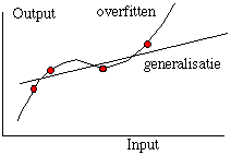 |
The number of units in a network is always a compromise between the generalization of many patterns and the learning of special patterns. The number of neurons required for a certain task is
statistically unpredictable. Two ideas have been developed to determine the number of neurons needed by the learning process itself:
1) A minimal network is trained, starting with simple, easily generalized patterns. Then more difficult problems are viewed, if these do not fit appropriately then extra neurons are added.
2) The patterns are placed in classes and for each class a network is taught. These networks are then combined into one network. Problems arise when combining results and removing redundant
parts.
|
Most of these methods do not have many known results. From a biological aspect, no or a restricted amount of new neurons are formed, for the synapses it looks as if these are formed. Of course
this says nothing about switching existing neurons to new tasks.
10.3 Back-propagation
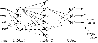 |
These are multi-layer feed-forward networks with back-propagation learning rules. Every neuron in a layer is connected to each of the neurons on the next layer, and there are no connections
between two neurons in one layer. The input layer gives the original input of every pattern to every neuron in the first hidden layer. The input values are often restricted to an interval of [0,1] or
[-1,1]. For most problems this doesn't matter much, but for some [-1,1] is more suitable. The neti of the hidden and output neurons is a weighted sum:
|
neti(t) =  j ( wj,i * oj ) +
  i
i
Here  i is often interpreted as a weight to a virtual neuron with a fixed output of 1.
The output function fi of every neuron has neti as input, and it must be possible to differentiate:
- linear f(x) =
 x
x
- logistic f(x) = logis(x) = 1 /(1 + e -
 x) (output between 0 and 1)
- tanh f(x) = tanh(x) = (e
 x - e -
 x) /(e
  x + e
-
 x) (between -1 and 1)
 is the slope, this is often constant and usually 1. Sometimes the slope is taught to each neuron individually.
Multiplying
  with a number coincides with dividing by all the weights and
  with the same number. So actually,
  can be taken fixed. However it is stated that by adjusting
  learning occurs faster.
The target value is the desired output for an output neuron for a particular learning pattern. For classification purposes there is often 1 output per class, with a high target value (0.8 to 1)
for input patterns in that class and a low (0 to 0.2, respectively -1.0 to -0.8) target value for the other input patterns. The output values must then be edited by another function to determine the
output class. For the approximation of a function with real values the output has a low linear activation function, while the hidden layers usually do not have a linear activation function at
all.
The next statement has been proven:
Given a  >0 and a L2 function f: [0,1]n -> Rm,
then there is a back-propagation network with one hidden layer that approximates f with a mean square error smaller than
  .
.
Essentially one hidden layer is enough, however the number of neurons in that layer can become enormous. It can be useful to try networks with more hidden layers, the total number of required
neurons could be less and then the net can work and learn faster.
Learning from a back-propagation net occurs as follows. First the weights and  s are initialized,
usually with random values often with a dispersal
  around 0. Then the learning patterns are offered and
the error function:
E = 1/2 p
p j ( o pj - t pj)2
calculated. The E(wij,  j) is minimized to all wij and
  j by a gradient descent method:
 wij= -
 E /
E /  wij with
  as the learning rate
For neuron j in the output layer the following is true:
- E /
E /  wij = - (
 E /
E /  netj ) (
 netj /
  wij)
wij)
=  p
(tpj - opj) (
 opj /
opj /  netj ) ohi
=  p
p  pj ohi (from the previous
layer)
for tanh():  pj = (tpj - opj)
1/2 (1-opj2)
for logis():  pj = (tpj -
opj) opj (1-opj)
For neuron i in the previous hidden layer, we can also determine - E /
E /  wki, keeping in mind that every oj is dependent on every ohi :
- E /
E /  wki =
wki =  p (
p ( j
j  pj wij ) (
 oi /
oi /  neti ) ohk
similar to the output layer but then with (tpj - opj) replaced by:  j
j  pj wij
The errors (tpj - opj) on the output neurons are thus divided over the hidden neurons lying before it, that is why it is called back-propagation. After
the input layer has been reached, the weights and the thresholds are adjusted and the learning patterns are offered again. For the thresholds  the same formulae hold because the thresholds can be interpreted as the weight to the virtual neuron always yielding an output of 1.
Often a large amount of iterations (epochs) are needed for each set of patterns. Learning continues until E is small enough, or even better yet, until the best results are attained using a
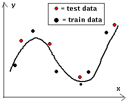
separate set of test patterns. By "over-learning" or over-specialization it can happen that the E decreases on the learning data while it increases on the test data.
 |
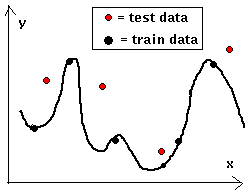 |
On the grounds of training data, the net on the left has learned the underlying trend in the curve well, the test data lies well in the neighborhood of the curve. To the right we see the results
of "over-learning", by taking the net on the left and teaching it more or by using a net with more hidden neurons. The training data lie precisely on the curve, but the test data exhibits large
deviations.
|
Afterwards a separate pattern verification set is used to see how well the net has "generalized". The learning, testing and verification set must be representative for the problem, attaining large
sets of representative patterns is a problem on its own.
 |
|
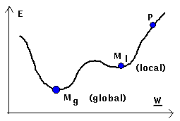
Next to "epoch" or "off-line" learning the weights can be changed after each pattern, named "on-line" learning and has a smaller learning rate. This is often faster (less epochs needed) and yields
better results with more complex problems and when the input patterns are noisy. This is because it is easier to jump over a local minimum. If we start in the picture on the side with a gradient
descent in p we reach the local minimum Ml and not the global minimum Mg.
|
To pass over smooth surfaces in E quickly and jump over shallow local minima, often a momentum term is used:
 wij(t) = -
 E /
E /  wij (t) +
 wij(t -1)
The number of neurons and layers, the values of the parameters (and possibly adjustments during the learning process)
and the initialization of the network must be determined experimentally.
There are many variations on the above mentioned "standard backprop", that sometimes yield better results than on-line learning
and often require less iterations. Well-known are "Quickprop" and
"RPROP", both regard E(wij) around the minimum as a parabola and look at the change in
sign of  E /
E /  wij to determine
  wij. They have 3 respectively 5 learning parameters of which the recommended ones often yield good results.
Learning patterns that have a "good" ( tj-oj <  ) output, leave out some
epochs, and thereby speed up the learning process. The ßj can also be learned for each neuron.
For the output neurons the following is true for tanh():
- E /
E / 
 j =
j =  p (tpj - opj) 1/2 (1-opj2) netj
10.4 Kohonen networks
With Kohonen networks, every neuron has a weighted vector w with the same dimension as the input patterns. For each supplied pattern p every neuron determines: || xp
-w || followed by determining the winning neuron m with the lowest match value. Weights are then adjusted depending on:
- winning neuron or not
 (t) (xp -wm) (winning neuron m moves to pattern p)
- distance to the winning neuron
- winning neuron has the same class as the learning pattern or not
With the Self Organizing Maps or Topology Preserving Maps the neurons are ordered in a 2-D matrix. Next to the winning neuron, neurons with a distance of r(t) are also adjusted according the
matrix:
 wi =
wi =  (t) (xp -wm) where
  (t) and r(t) decrease
linearly with the number of epochs.
Clusters of patterns in the feature space are placed on a cluster of one or more neurons in the matrix. This is an unsupervised learning method; one must yet determine what the belonging clusters
in the matrix mean in the coinciding feature space.
The Ritter∓Schulten variation is used a lo. Here every neuron is adjusted by:
 wi =
wi =  (t) (xp -wm) exp (-afst(i,m)2 /
  (t)2 ) with afst() the Euclidic distance in the 2-D matrix
 (t) and
  (t) are
multiplied by c < 1 per epoch
 |
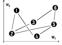 |
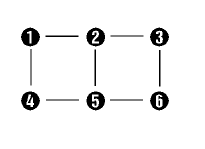
To the left we see 6 Kohonen neurons ordered in a 2 by 3, 2-D matrix. To the right the initial positions of the neurons in the weighted space are shown, which are for example chosen randomly.
|
 |
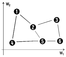 |
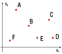
To the left the positions of 6 input patterns are shown, or rather the center of the 6 classes of the input patterns. A well-trained SOM then attains the positions in the feature space such as
shown on the right. These are centered on the positions of the clusters, and clusters lying close to each other in the feature space end up on neurons which also lie close to each other in the
matrix. The topology of the feature space can be found in the matrix space.
|
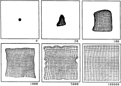 |
Here we took randomly chosen positions in the 2-D unit-square as input patterns.
The neurons are initialized with small values around the 0. We see that the Kohonen neurons slowly develop to regular positions in the unit-square.
|
With Learning Vector Quantization (LVQ), several neurons from each class are taken and initialized (a supervised method), for example spread out around the average of the learning pattern. The
winning neuron is adjusted:
 wi = ±
 (t) (xp -wm) (+ same class, - other class)
Besides only the winning neuron, using LVQ2 and 3, also the second best is taken into account.
10.5 Classical pattern-recognition methods
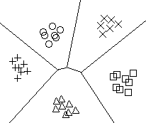 |
These try to find discriminating functions to divide classes:
di(x) > dj(x) for j  i when pattern x
belongs to class i i when pattern x
belongs to class i
With the minimum distance or minimum mean classifier, every class attains a prototype vector: mi =  x x chi x / Ni chi x / Ni
An input vector x attains class i if ||x-mi|| is minimal, the coinciding discriminating function is then: di(x) =
xTmi - 1/2 miTmi (fig. 12.6)
|
The probability that pattern x comes from the class  i, is indicated by: p(
 i | x). If a classifier decides that x comes from
  j while it actually comes from
  i, there is a loss or error in the classification which can be indicated by Lij . Because x can belong to each of the present M classes, the average loss when x is
credited to
  j is:
j is:
crj(x) =  k Lkj p(
 k | x)
Using Bayes theorem: p( | b) = p(
 ) p(b |
  ) / p(b) :
crj(x) = (1 / p(x))  k
Lkj p(x |
  k) p(
k) p( k)
k)
Because p(x) is a positive value this term is left out: rj(x) = k
Lkj p(x |
  k) p(
k) p( k) (average risk or loss)
A Bayes classifier adds x to class  j if rj(x) <
ri(x) for all i
  j and thus minimizes the total average loss caused by
incorrect classifications.
In many problems the loss is 0 for a correct decision and 1 for an incorrect decision:
Lkj = 1 -  kj thus: rj(x) =
 k (1 -
  kj ) p(x |
  k) p(
k) p( k) = p(x) - p(x |
  j) p(
j) p( j)
j)
This coincides with the decision function: dj(x) = p(x |  j)p(
j)p( j)
j)
To be able to construct a Bayes classifier we need knowledge about the probabilities of the distributions patterns in the classes which are present, and a loss function relevant to that particular
problem. Often Gaussian distributions are assumed [12.10] or other functions which can be calculated easily, and where the parameters of the functions can be determined with a certain precision from
the learning patterns present.
For many medical and also other applications Lij  Lji. While
testing on the presence of a certain disease it is often less dramatic for a healthy person to be diagnosed as sick rather than a sick person being diagnosed as healthy. With a "false positive"
decision the following and other tests will indicate the illness not to be present, with a "false negative" decision the patient goes home and the illness can develop further.
There are many, however not always known, resemblances between neural networks and classical statistical pattern recognition methods. Attractive for neural networks is that these work with
examples and without the use of "higher order" knowledge of the underlying problem. When the results of the classification are sufficient (hopefully, because there is no guarantee that a problem is
taught), we have enough information unless one wants to include "higher order" information (distributions, etc.) about the underlying problem. This information has been hidden in the large amount of
weights and is difficult to retrieve. Using domain knowledge can often lead to better solutions.
Updated on April 4th 2003 by Theo Schouten.